Добавить распространенная легенда для комбинированной ggplots
у меня есть два ggplots, которые я выравниваю по горизонтали с grid.arrange. Я просмотрел много сообщений на форуме, но все, что я пытаюсь, похоже, команды, которые теперь обновляются и называются чем-то другим.
мои данные выглядит так:
# Data plot 1

        axis1     axis2

group1 -0.212201  0.358867

group2 -0.279756 -0.126194

group3  0.186860 -0.203273

group4  0.417117 -0.002592

group1 -0.212201  0.358867

group2 -0.279756 -0.126194

group3  0.186860 -0.203273

group4  0.186860 -0.203273


# Data plot 2

        axis1     axis2

group1  0.211826 -0.306214

group2 -0.072626  0.104988

group3 -0.072626  0.104988

group4 -0.072626  0.104988

group1  0.211826 -0.306214

group2 -0.072626  0.104988

group3 -0.072626  0.104988

group4 -0.072626  0.104988


#And I run this:

library(ggplot2)

library(gridExtra)


groups=c('group1','group2','group3','group4','group1','group2','group3','group4')


x1=data1[,1]

y1=data1[,2]


x2=data2[,1]

y2=data2[,2]


p1=ggplot(data1, aes(x=x1, y=y1,colour=groups)) + geom_point(position=position_jitter(w=0.04,h=0.02),size=1.8)


p2=ggplot(data2, aes(x=x2, y=y2,colour=groups)) + geom_point(position=position_jitter(w=0.04,h=0.02),size=1.8)


#Combine plots

p3=grid.arrange(

p1 + theme(legend.position="none"), p2+ theme(legend.position="none"), nrow=1, widths = unit(c(10.,10), "cm"), heights = unit(rep(8, 1), "cm")))
Как я могу извлечь легенду из любого из этих участков и добавить ее в нижнюю/центральную часть объединенного участка?
7 ответов:
Обновление 2015-Февраль
посмотреть ответ Стивена ниже
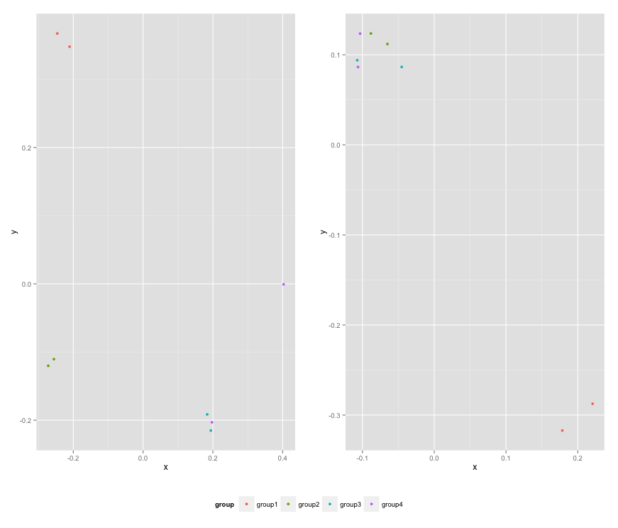
df1 <- read.table(text="group   x     y
group1 -0.212201  0.358867
group2 -0.279756 -0.126194
group3  0.186860 -0.203273
group4  0.417117 -0.002592
group1 -0.212201  0.358867
group2 -0.279756 -0.126194
group3  0.186860 -0.203273
group4  0.186860 -0.203273",header=TRUE)

df2 <- read.table(text="group   x     y
group1  0.211826 -0.306214
group2 -0.072626  0.104988
group3 -0.072626  0.104988
group4 -0.072626  0.104988
group1  0.211826 -0.306214
group2 -0.072626  0.104988
group3 -0.072626  0.104988
group4 -0.072626  0.104988",header=TRUE)


library(ggplot2)
library(gridExtra)

p1 <- ggplot(df1, aes(x=x, y=y,colour=group)) + geom_point(position=position_jitter(w=0.04,h=0.02),size=1.8) + theme(legend.position="bottom")

p2 <- ggplot(df2, aes(x=x, y=y,colour=group)) + geom_point(position=position_jitter(w=0.04,h=0.02),size=1.8)

#extract legend
#https://github.com/hadley/ggplot2/wiki/Share-a-legend-between-two-ggplot2-graphs
g_legend<-function(a.gplot){
  tmp <- ggplot_gtable(ggplot_build(a.gplot))
  leg <- which(sapply(tmp$grobs, function(x) x$name) == "guide-box")
  legend <- tmp$grobs[[leg]]
  return(legend)}

mylegend<-g_legend(p1)

p3 <- grid.arrange(arrangeGrob(p1 + theme(legend.position="none"),
                         p2 + theme(legend.position="none"),
                         nrow=1),
             mylegend, nrow=2,heights=c(10, 1))
вот результирующий график:
ответ Роланда нуждается в обновлении. Смотрите: https://github.com/hadley/ggplot2/wiki/Share-a-legend-between-two-ggplot2-graphs
этот метод был обновлен для ggplot2 v1.0.0.
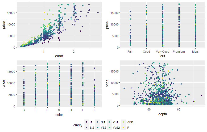
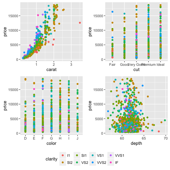
library(ggplot2)
library(gridExtra)
library(grid)


grid_arrange_shared_legend <- function(...) {
    plots <- list(...)
    g <- ggplotGrob(plots[[1]] + theme(legend.position="bottom"))$grobs
    legend <- g[[which(sapply(g, function(x) x$name) == "guide-box")]]
    lheight <- sum(legend$height)
    grid.arrange(
        do.call(arrangeGrob, lapply(plots, function(x)
            x + theme(legend.position="none"))),
        legend,
        ncol = 1,
        heights = unit.c(unit(1, "npc") - lheight, lheight))
}

dsamp <- diamonds[sample(nrow(diamonds), 1000), ]
p1 <- qplot(carat, price, data=dsamp, colour=clarity)
p2 <- qplot(cut, price, data=dsamp, colour=clarity)
p3 <- qplot(color, price, data=dsamp, colour=clarity)
p4 <- qplot(depth, price, data=dsamp, colour=clarity)
grid_arrange_shared_legend(p1, p2, p3, p4)
обратите внимание на отсутствие
ggplot_gtableиggplot_build.ggplotGrobиспользуется вместо этого. Этот пример немного более запутан, чем приведенное выше решение, но он все равно решил его для меня.
вы также можете использовать ggarrange С ggpubr пакет и набор " общие.legend = TRUE":
library(ggpubr)

dsamp <- diamonds[sample(nrow(diamonds), 1000), ]
p1 <- qplot(carat, price, data = dsamp, colour = clarity)
p2 <- qplot(cut, price, data = dsamp, colour = clarity)
p3 <- qplot(color, price, data = dsamp, colour = clarity)
p4 <- qplot(depth, price, data = dsamp, colour = clarity)

ggarrange(p1, p2, p3, p4, ncol=2, nrow=2, common.legend = TRUE, legend="bottom")
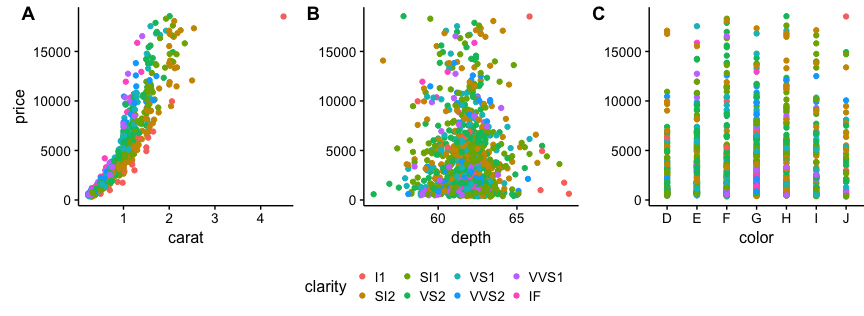
Я предлагаю использовать cowplot. От их R виньетка:
# load cowplot
library(cowplot)

# down-sampled diamonds data set
dsamp <- diamonds[sample(nrow(diamonds), 1000), ]

# Make three plots.
# We set left and right margins to 0 to remove unnecessary spacing in the
# final plot arrangement.
p1 <- qplot(carat, price, data=dsamp, colour=clarity) +
   theme(plot.margin = unit(c(6,0,6,0), "pt"))
p2 <- qplot(depth, price, data=dsamp, colour=clarity) +
   theme(plot.margin = unit(c(6,0,6,0), "pt")) + ylab("")
p3 <- qplot(color, price, data=dsamp, colour=clarity) +
   theme(plot.margin = unit(c(6,0,6,0), "pt")) + ylab("")

# arrange the three plots in a single row
prow <- plot_grid( p1 + theme(legend.position="none"),
           p2 + theme(legend.position="none"),
           p3 + theme(legend.position="none"),
           align = 'vh',
           labels = c("A", "B", "C"),
           hjust = -1,
           nrow = 1
           )

# extract the legend from one of the plots
# (clearly the whole thing only makes sense if all plots
# have the same legend, so we can arbitrarily pick one.)
legend_b <- get_legend(p1 + theme(legend.position="bottom"))

# add the legend underneath the row we made earlier. Give it 10% of the height
# of one plot (via rel_heights).
p <- plot_grid( prow, legend_b, ncol = 1, rel_heights = c(1, .2))
p
@Giuseppe, вы можете рассмотреть это для гибкой спецификации расположения участков (изменено от здесь):
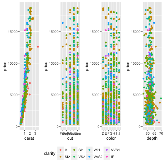
library(ggplot2)
library(gridExtra)
library(grid)

grid_arrange_shared_legend <- function(..., nrow = 1, ncol = length(list(...)), position = c("bottom", "right")) {

  plots <- list(...)
  position <- match.arg(position)
  g <- ggplotGrob(plots[[1]] + theme(legend.position = position))$grobs
  legend <- g[[which(sapply(g, function(x) x$name) == "guide-box")]]
  lheight <- sum(legend$height)
  lwidth <- sum(legend$width)
  gl <- lapply(plots, function(x) x + theme(legend.position = "none"))
  gl <- c(gl, nrow = nrow, ncol = ncol)

  combined <- switch(position,
                     "bottom" = arrangeGrob(do.call(arrangeGrob, gl),
                                            legend,
                                            ncol = 1,
                                            heights = unit.c(unit(1, "npc") - lheight, lheight)),
                     "right" = arrangeGrob(do.call(arrangeGrob, gl),
                                           legend,
                                           ncol = 2,
                                           widths = unit.c(unit(1, "npc") - lwidth, lwidth)))
  grid.newpage()
  grid.draw(combined)

}
Дополнительные параметры
nrowиncolконтролируйте расположение расположенных участков:dsamp <- diamonds[sample(nrow(diamonds), 1000), ] p1 <- qplot(carat, price, data = dsamp, colour = clarity) p2 <- qplot(cut, price, data = dsamp, colour = clarity) p3 <- qplot(color, price, data = dsamp, colour = clarity) p4 <- qplot(depth, price, data = dsamp, colour = clarity) grid_arrange_shared_legend(p1, p2, p3, p4, nrow = 1, ncol = 4) grid_arrange_shared_legend(p1, p2, p3, p4, nrow = 2, ncol = 2)
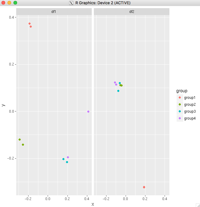
Если вы строите одни и те же переменные на обоих участках, самым простым способом было бы объединить фреймы данных в один, а затем использовать facet_wrap.
для примера:
big_df <- rbind(df1,df2)

big_df <- data.frame(big_df,Df = rep(c("df1","df2"),
times=c(nrow(df1),nrow(df2))))

ggplot(big_df,aes(x=x, y=y,colour=group))
+ geom_point(position=position_jitter(w=0.04,h=0.02),size=1.8)
+ facet_wrap(~Df)
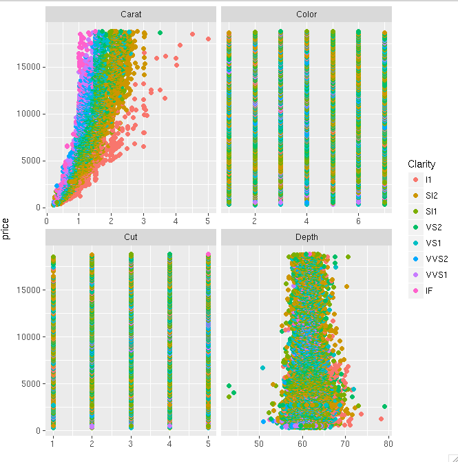
другой пример использования набора данных diamonds. Это показывает, что вы даже можете заставить его работать, если у вас есть только одна переменная, общая для ваших графиков.
diamonds_reshaped <- data.frame(price = diamonds$price,
independent.variable = c(diamonds$carat,diamonds$cut,diamonds$color,diamonds$depth),
Clarity = rep(diamonds$clarity,times=4),
Variable.name = rep(c("Carat","Cut","Color","Depth"),each=nrow(diamonds)))

ggplot(diamonds_reshaped,aes(independent.variable,price,colour=Clarity)) +
geom_point(size=2) + facet_wrap(~Variable.name,scales="free_x") +
xlab("")
только хитрая вещь с второй пример заключается в том, что факторные переменные принудительно преобразуются в числовые, когда вы объединяете все в один фрейм данных. Поэтому в идеале, вы будете делать это в основном тогда, когда все переменные относятся к одному типу.
@Guiseppe:
Я понятия не имею о гробах и т. д. Вообще, но я взломал решение для двух участков, должно быть возможно расширить до произвольного числа, но его не в сексуальной функции:
plots <- list(p1, p2)
g <- ggplotGrob(plots[[1]] + theme(legend.position="bottom"))$grobs
legend <- g[[which(sapply(g, function(x) x$name) == "guide-box")]]
lheight <- sum(legend$height)
tmp <- arrangeGrob(p1 + theme(legend.position = "none"), p2 + theme(legend.position = "none"), layout_matrix = matrix(c(1, 2), nrow = 1))
grid.arrange(tmp, legend, ncol = 1, heights = unit.c(unit(1, "npc") - lheight, lheight))
Comments