Анализ основных компонентов в Python

Question

Анализ основных компонентов в Python

Я хотел бы использовать анализ главных компонентов (PCA) для уменьшения размерности. У numpy или scipy уже есть это, или мне нужно свернуть свой собственный с помощью numpy.linalg.eigh?

Я не просто хочу использовать сингулярную декомпозицию (SVD), потому что мои входные данные довольно многомерны (~460 измерений), поэтому я думаю, что SVD будет медленнее, чем вычисление собственных векторов ковариационной матрицы.

Я надеялся найти готовую, отлаженную реализацию это уже делает правильные решения о том, когда использовать какой метод, и который, возможно, делает другие оптимизации, о которых я не знаю.

910 10

python numpy scipy pca

10 ответов:

Comments

Ничего не найдено.

ChristopheD · Accepted Answer · 2010-09-03 14:40:33

вы могли бы взглянуть на MDP.

У меня не было возможности проверить его самостоятельно, но я закладки именно для функциональности PCA.

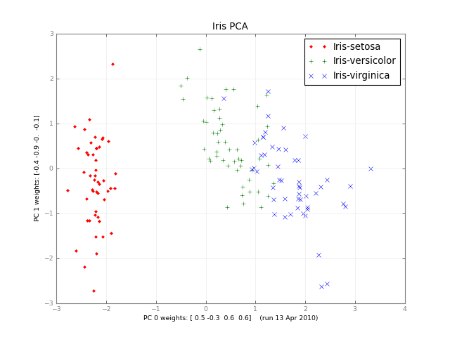
denis · Accepted Answer · 2017-03-21 14:05:55

месяцы спустя, вот небольшой класс PCA, и изображение:

#!/usr/bin/env python
""" a small class for Principal Component Analysis
Usage:
    p = PCA( A, fraction=0.90 )
In:
    A: an array of e.g. 1000 observations x 20 variables, 1000 rows x 20 columns
    fraction: use principal components that account for e.g.
        90 % of the total variance

Out:
    p.U, p.d, p.Vt: from numpy.linalg.svd, A = U . d . Vt
    p.dinv: 1/d or 0, see NR
    p.eigen: the eigenvalues of A*A, in decreasing order (p.d**2).
        eigen[j] / eigen.sum() is variable j's fraction of the total variance;
        look at the first few eigen[] to see how many PCs get to 90 %, 95 % ...
    p.npc: number of principal components,
        e.g. 2 if the top 2 eigenvalues are >= `fraction` of the total.
        It's ok to change this; methods use the current value.

Methods:
    The methods of class PCA transform vectors or arrays of e.g.
    20 variables, 2 principal components and 1000 observations,
    using partial matrices U' d' Vt', parts of the full U d Vt:
    A ~ U' . d' . Vt' where e.g.
        U' is 1000 x 2
        d' is diag([ d0, d1 ]), the 2 largest singular values
        Vt' is 2 x 20.  Dropping the primes,

    d . Vt      2 principal vars = p.vars_pc( 20 vars )
    U           1000 obs = p.pc_obs( 2 principal vars )
    U . d . Vt  1000 obs, p.obs( 20 vars ) = pc_obs( vars_pc( vars ))
        fast approximate A . vars, using the `npc` principal components

    Ut              2 pcs = p.obs_pc( 1000 obs )
    V . dinv        20 vars = p.pc_vars( 2 principal vars )
    V . dinv . Ut   20 vars, p.vars( 1000 obs ) = pc_vars( obs_pc( obs )),
        fast approximate Ainverse . obs: vars that give ~ those obs.


Notes:
    PCA does not center or scale A; you usually want to first
        A -= A.mean(A, axis=0)
        A /= A.std(A, axis=0)
    with the little class Center or the like, below.

See also:
    http://en.wikipedia.org/wiki/Principal_component_analysis
    http://en.wikipedia.org/wiki/Singular_value_decomposition
    Press et al., Numerical Recipes (2 or 3 ed), SVD
    PCA micro-tutorial
    iris-pca .py .png

"""

from __future__ import division
import numpy as np
dot = np.dot
    # import bz.numpyutil as nu
    # dot = nu.pdot

__version__ = "2010-04-14 apr"
__author_email__ = "denis-bz-py at t-online dot de"

#...............................................................................
class PCA:
    def __init__( self, A, fraction=0.90 ):
        assert 0 <= fraction <= 1
            # A = U . diag(d) . Vt, O( m n^2 ), lapack_lite --
        self.U, self.d, self.Vt = np.linalg.svd( A, full_matrices=False )
        assert np.all( self.d[:-1] >= self.d[1:] )  # sorted
        self.eigen = self.d**2
        self.sumvariance = np.cumsum(self.eigen)
        self.sumvariance /= self.sumvariance[-1]
        self.npc = np.searchsorted( self.sumvariance, fraction ) + 1
        self.dinv = np.array([ 1/d if d > self.d[0] * 1e-6  else 0
                                for d in self.d ])

    def pc( self ):
        """ e.g. 1000 x 2 U[:, :npc] * d[:npc], to plot etc. """
        n = self.npc
        return self.U[:, :n] * self.d[:n]

    # These 1-line methods may not be worth the bother;
    # then use U d Vt directly --

    def vars_pc( self, x ):
        n = self.npc
        return self.d[:n] * dot( self.Vt[:n], x.T ).T  # 20 vars -> 2 principal

    def pc_vars( self, p ):
        n = self.npc
        return dot( self.Vt[:n].T, (self.dinv[:n] * p).T ) .T  # 2 PC -> 20 vars

    def pc_obs( self, p ):
        n = self.npc
        return dot( self.U[:, :n], p.T )  # 2 principal -> 1000 obs

    def obs_pc( self, obs ):
        n = self.npc
        return dot( self.U[:, :n].T, obs ) .T  # 1000 obs -> 2 principal

    def obs( self, x ):
        return self.pc_obs( self.vars_pc(x) )  # 20 vars -> 2 principal -> 1000 obs

    def vars( self, obs ):
        return self.pc_vars( self.obs_pc(obs) )  # 1000 obs -> 2 principal -> 20 vars


class Center:
    """ A -= A.mean() /= A.std(), inplace -- use A.copy() if need be
        uncenter(x) == original A . x
    """
        # mttiw
    def __init__( self, A, axis=0, scale=True, verbose=1 ):
        self.mean = A.mean(axis=axis)
        if verbose:
            print "Center -= A.mean:", self.mean
        A -= self.mean
        if scale:
            std = A.std(axis=axis)
            self.std = np.where( std, std, 1. )
            if verbose:
                print "Center /= A.std:", self.std
            A /= self.std
        else:
            self.std = np.ones( A.shape[-1] )
        self.A = A

    def uncenter( self, x ):
        return np.dot( self.A, x * self.std ) + np.dot( x, self.mean )


#...............................................................................
if __name__ == "__main__":
    import sys

    csv = "iris4.csv"  # wikipedia Iris_flower_data_set
        # 5.1,3.5,1.4,0.2  # ,Iris-setosa ...
    N = 1000
    K = 20
    fraction = .90
    seed = 1
    exec "\n".join( sys.argv[1:] )  # N= ...
    np.random.seed(seed)
    np.set_printoptions( 1, threshold=100, suppress=True )  # .1f
    try:
        A = np.genfromtxt( csv, delimiter="," )
        N, K = A.shape
    except IOError:
        A = np.random.normal( size=(N, K) )  # gen correlated ?

    print "csv: %s  N: %d  K: %d  fraction: %.2g" % (csv, N, K, fraction)
    Center(A)
    print "A:", A

    print "PCA ..." ,
    p = PCA( A, fraction=fraction )
    print "npc:", p.npc
    print "% variance:", p.sumvariance * 100

    print "Vt[0], weights that give PC 0:", p.Vt[0]
    print "A . Vt[0]:", dot( A, p.Vt[0] )
    print "pc:", p.pc()

    print "\nobs <-> pc <-> x: with fraction=1, diffs should be ~ 0"
    x = np.ones(K)
    # x = np.ones(( 3, K ))
    print "x:", x
    pc = p.vars_pc(x)  # d' Vt' x
    print "vars_pc(x):", pc
    print "back to ~ x:", p.pc_vars(pc)

    Ax = dot( A, x.T )
    pcx = p.obs(x)  # U' d' Vt' x
    print "Ax:", Ax
    print "A'x:", pcx
    print "max |Ax - A'x|: %.2g" % np.linalg.norm( Ax - pcx, np.inf )

    b = Ax  # ~ back to original x, Ainv A x
    back = p.vars(b)
    print "~ back again:", back
    print "max |back - x|: %.2g" % np.linalg.norm( back - x, np.inf )

# end pca.py

ali_m · Accepted Answer · 2015-12-01 17:18:48

PCA с помощью numpy.linalg.svd супер просто. Вот простой пример:

import numpy as np
import matplotlib.pyplot as plt
from scipy.misc import lena

# the underlying signal is a sinusoidally modulated image
img = lena()
t = np.arange(100)
time = np.sin(0.1*t)
real = time[:,np.newaxis,np.newaxis] * img[np.newaxis,...]

# we add some noise
noisy = real + np.random.randn(*real.shape)*255

# (observations, features) matrix
M = noisy.reshape(noisy.shape[0],-1)

# singular value decomposition factorises your data matrix such that:
# 
#   M = U*S*V.T     (where '*' is matrix multiplication)
# 
# * U and V are the singular matrices, containing orthogonal vectors of
#   unit length in their rows and columns respectively.
#
# * S is a diagonal matrix containing the singular values of M - these 
#   values squared divided by the number of observations will give the 
#   variance explained by each PC.
#
# * if M is considered to be an (observations, features) matrix, the PCs
#   themselves would correspond to the rows of S^(1/2)*V.T. if M is 
#   (features, observations) then the PCs would be the columns of
#   U*S^(1/2).
#
# * since U and V both contain orthonormal vectors, U*V.T is equivalent 
#   to a whitened version of M.

U, s, Vt = np.linalg.svd(M, full_matrices=False)
V = Vt.T

# PCs are already sorted by descending order 
# of the singular values (i.e. by the
# proportion of total variance they explain)

# if we use all of the PCs we can reconstruct the noisy signal perfectly
S = np.diag(s)
Mhat = np.dot(U, np.dot(S, V.T))
print "Using all PCs, MSE = %.6G" %(np.mean((M - Mhat)**2))

# if we use only the first 20 PCs the reconstruction is less accurate
Mhat2 = np.dot(U[:, :20], np.dot(S[:20, :20], V[:,:20].T))
print "Using first 20 PCs, MSE = %.6G" %(np.mean((M - Mhat2)**2))

fig, [ax1, ax2, ax3] = plt.subplots(1, 3)
ax1.imshow(img)
ax1.set_title('true image')
ax2.imshow(noisy.mean(0))
ax2.set_title('mean of noisy images')
ax3.imshow((s[0]**(1./2) * V[:,0]).reshape(img.shape))
ax3.set_title('first spatial PC')
plt.show()

Noam Peled · Accepted Answer · 2013-08-22 22:58:02

вы можете использовать sklearn:

import sklearn.decomposition as deco
import numpy as np

x = (x - np.mean(x, 0)) / np.std(x, 0) # You need to normalize your data first
pca = deco.PCA(n_components) # n_components is the components number after reduction
x_r = pca.fit(x).transform(x)
print ('explained variance (first %d components): %.2f'%(n_components, sum(pca.explained_variance_ratio_)))

tom10 · Accepted Answer · 2014-02-13 23:44:00

matplotlib.mlab есть реализация PCA.

31

2014-02-13 23:44:00

dwf · Accepted Answer · 2009-11-15 04:59:26

SVD должен работать нормально с 460 размерами. Это занимает около 7 секунд на моем нетбуке Atom. Метод eig() принимает больше время (как и должно быть, он использует больше операций с плавающей запятой) и почти всегда будет менее точным.

Если у вас меньше 460 примеров, то вы хотите диагонализировать матрицу рассеяния (x - datamean)^T(X - mean), предполагая, что ваши точки данных являются столбцами, а затем умножить налево (x-datamean). Это может будет быстрее в том случае, когда у вас больше измерений, чем данные.

Anony-Mousse · Accepted Answer · 2014-05-26 16:55:54

вы можете довольно легко "свернуть" свой собственный с помощью scipy.linalg (предполагая предварительно центрированный набор данных data):
covmat = data.dot(data.T)
evs, evmat = scipy.linalg.eig(covmat)
затем evs - твои собственные, и evmat ваша матрица проекции.

если вы хотите сохранить d размеры, используйте первый d собственные значения и первый d собственные векторы.

учитывая, что scipy.linalg имеет декомпозицию и numpy матричные умножения, что еще вам нужно?

sunqiang · Accepted Answer · 2009-11-14 02:29:28

Я только что дочитал книгу Машинное Обучение: Алгоритмическая Перспектива. Все примеры кода в книге были написаны на Python (и почти с Numpy). Фрагмент кода анализ основных компонентов chatper10.2 может быть, стоит читать. Он использует numpy.linalg.Эйг.
Кстати, я думаю, что SVD может обрабатывать размеры 460 * 460 очень хорошо. Я рассчитал 6500 * 6500 SVD с numpy / scipy.linalg.svd на очень старом ПК: Pentium III 733mHz. Если честно, сценарий требует много памяти(около 1.xG) и много времени(около 30 минут), чтобы получить результат SVD. Но я думаю, что 460*460 на современном ПК не будет большой проблемой, если вам не нужно делать SVD огромное количество раз.

Nicolas Barbey · Accepted Answer · 2012-08-06 16:39:37

вам не нужно полное сингулярное разложение (SVD) при нем вычисляются все собственные значения и собственные векторы и могут быть запретительными для больших матриц. составляющей и его разреженный модуль обеспечивают общие линейные функции альгребры, работающие как на разреженных, так и на плотных матрицах, среди которых есть семейство функций eig* :

http://docs.scipy.org/doc/scipy/reference/sparse.linalg.html#matrix-factorizations

Scikit-learn предоставляет реализация Python PCA которые пока поддерживают только плотные матрицы.

часы работы :
In [1]: A = np.random.randn(1000, 1000)

In [2]: %timeit scipy.sparse.linalg.eigsh(A)
1 loops, best of 3: 802 ms per loop

In [3]: %timeit np.linalg.svd(A)
1 loops, best of 3: 5.91 s per loop

rcs · Accepted Answer · 2009-11-13 20:42:57

здесь является еще одной реализацией модуля PCA для python с использованием NumPy, scipy и C-расширений. Модуль выполняет PCA, используя либо SVD, либо алгоритм NIPALS (нелинейный итерационный частичный наименьший квадрат), который реализован в C.